Description
The functions that form this module take the emission sets per
TM5-FASST region and year generated in Module 1 (by
m1_emissions_rescale), and estimate the fine particulate
matter (PM2.5) and ozone (O3) concentration levels for each period and
TM5-FASST region. In particular the package reports the following range
of PM2.5 and O3 indicators:
- Fine particulate matter (PM2.5) concentration levels
(
m2_get_conc_pm25) - Raw ozone concentration levels (
m2_get_conc_o3) - Maximum 6-monthly running average of daily maximum hourly O3 (M6M,
also known as 6mDMA1) (
m2_get_conc_m6m). This indicator is used to compute health impacts attributable to exposure to ozone (see Jerret et al 2009)
The module includes two additional functions to estimate crop losses
associated with high ozone concentration levels, suing two different
mettrics described in Van
Dingenen et al 2009: * Accumulated daytime hourly O3 concentration
above a threshold of 40 ppbV (AOT40) (m2_get_conc_aot40) *
Seasonal mean daytime O3 concentration (m2_get_conc_mi)
The code below shows an example to get PM2.5 concentration levels:
library(rfasst)
library(magrittr)

 db_path<-"path_to_your_gcam_database"
 query_path<-"path_to_your_gcam_queries_file"
 db_name<-"name of the database"
 prj_name <- "Name of the rgcam project" # This can be an existing project, or, if not, this will be the name
 rdata_name <- "Name of the RData file." #It must contain the queries in a list
 scen_name<-"name of the GCAM scenario"
 queries<-"Name of the query file" # (the package includes a default query file that includes all the queries required in every function in the packae, "queries_rfasst.xml")
 final_db_year <- "Final year in the GCAM database" # This allows to process databases with user-defined "stop periods"
 saveOutput <- T # Writes the files.By default = T
 map <- T # Produce the maps. By default = F
 recompute <- F  # If set to T, recomputes the function output. Otherwise, if the output was already computed once, it uses that value and avoids repeating computations. By default = F


    m2_get_conc_pm25(db_path, query_path, db_name, prj_name, rdata_name, scen_name, queries,
saveOutput = F, final_db_year = final_db_year, recompute = recompute) map = T parameter, and
they will be generated and stored in the corresponding output
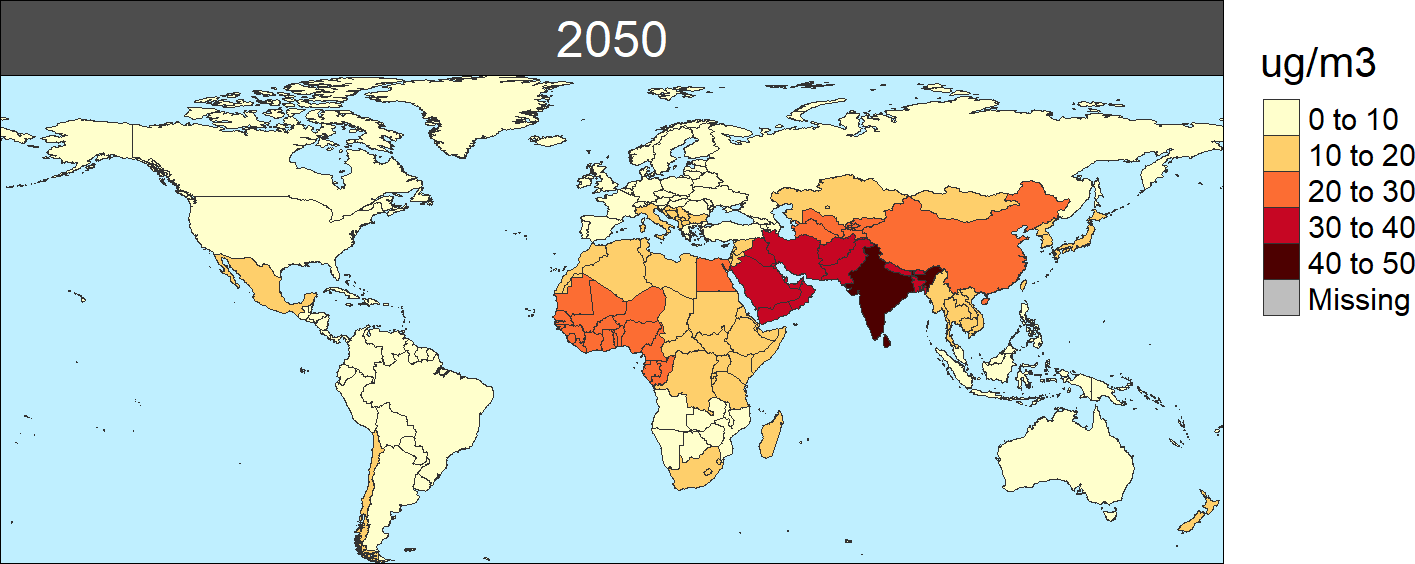
sub-directory. As an example for this module, the following map shows
the PM2.5 concentrations in 2050:
PM2.5 concntration by region in 2050 (ug/m3)

As indicated in the documentation of TM5-FASST Van Dingenen et al 2018,estimates of PM2.5 and O3 concentration levels in a receptor region driven by the emissions of different precursors in different sources are based on parametrizations of meteorology and atmospheric chemistry drawn from the more complex TM5 model. In summary, concentration of a pollutant , in region , from all the precursors () emitted in all regions (), is calculated as:
is the base-run concentration level of pollutant j in region y, pre-computed with TM5.
are the base-run precursor i emissions in region
= the –to- source-receptor coefficient for source region and receptor region y, pre-computed from a 20% emission reduction of component i in region relative to the base-run
are the emissions of precursor i in region in the analyzed scenario.
Following this equation, base-run emissions and concentrations, and source-receptor coefficient matrixes need to be combined with emissions pathways for the analyzed scenario. The package includes the following input information:
- Source-receptor coefficient matrixes (SRC):
- PM2.5 Source-receptor matrixes:
- SO4: SO2, NOx and NH3
- NO3: NOx, SO2, and NH3
- NH4: NH3, NOx and SO2
- BC: BC_POP
- POM: POM_POP
- O3 Source-receptor matrixes:
- For O3 exposure (O3): NOx, NMVOC and SO2
- For health calculations: M6M (6mDMA1): NOx, NMVOC, SO2 and CH4
- For agricultural damages:
- AOT40: NOx, NMVOC, SO2 and CH4
- Mi (M7 and M12): NOx, NMVOC, SO2 and CH4
- PM2.5 Source-receptor matrixes:
The package also includes the base emission and concentration levels for all these indicators.
In addition, primary PM2.5 emissions (BC and POM) are assumed to have a more direct influence in urban (more dense) areas, so the emission-concentration relation for these two pollutants is modified using adjustment coefficients that are included in the package.
Downscaling PM2.5 concentrations
The new release of rfasst (rfasst-v2.0) allows the user to get high-resolution (0.01 x 0.01 km) gridded concentration maps. The gridded PM2.5 maps are based on a static downscaling approach, based on observed PM2.5 data from Hammer et al 2020. As indicated in their publication, this dataset includes “annual concentrations (micrograms per cubic meter) of all composition ground-level fine particulate matter (PM2.5). This data set combines”AOD retrievals from multiple satellite algorithms including the NASA MODerate resolution Imaging Spectroradiometer Collection 6.1 (MODIS C6.1), Multi-angle Imaging SpectroRadiometer Version 23 (MISRv23), MODIS Multi-Angle Implementation of Atmospheric Correction Collection 6 (MAIAC C6), and the Sea-Viewing Wide Field-of-View Sensor (SeaWiFS) Deep Blue Version 4.”
We use this data to compute static “grid-to-region” coefficients that
are saved as a raster file and provided with the package
(pm25_weights_rast_rfasstReg).
Once the region-level PM2.5 concentration levels are calculated
(using the m2_get_conc_pm25 function), the obtained
dataframe can be rasterized to a 0.01 x 0.01 resolution grid map.
Then, we combine the rasterized output with the pre-computed grid-to-region downscaling coefficients to obtain the final gridded output.
The downscaling procedure can be activated by setting the parameter
downscale = T. This requires significantly more computing
time so it is set to F by default. In addition, the user
can write the produced raster file as a georeferenced “tiff” file by
setting saveRaster_grid = T (with the associated increase
in the computing time).
Finally, the updated tool also enables to re-aggregate the gridded
output to a new resolution of interest for the user. In this version,
the tool only includes to re-aggregate gridded results to the “NUTS3”
aggregation by the European Commission. In order to get additional
resolutions, the user would need to load their shape file (as a
SpatVector object) and make some changes in the corresponding code
(Lines 493-527, m2_conc.R). Future model version will try
to make this procedure more user-friendly, which is a challenge due to
the large size of these shape files. The re-aggregation of the gridded
data to new resolutions can be activated with the following boolean:
agg_grid = T. Likewise, the re-aggregated results can be
written as a .csv file by setting
save_AggGrid = T.
An example is provided in the code below:
library(rfasst)
library(magrittr)

 db_path<-"path_to_your_gcam_database"
 query_path<-"path_to_your_gcam_queries_file"
 db_name<-"name of the database"
 prj_name <- "Name of the rgcam project" # This can be an existing project, or, if not, this will be the name
 rdata_name <- "Name of the RData file." #It must contain the queries in a list
 scen_name<-"name of the GCAM scenario"
 queries<-"Name of the query file" # (the package includes a default query file that includes all the queries required in every function in the packae, "queries_rfasst.xml")
 final_db_year <- "Final year in the GCAM database" # This allows to process databases with user-defined "stop periods"
 saveOutput <- T # Writes the files.By default = T
 map <- T # Produce the maps. By default = F
 recompute <- F  # If set to T, recomputes the function output. Otherwise, if the output was already computed once, it uses that value and avoids repeating computations. By default = F
 downscale <- T  # If set to T, produces gridded PM2.5 outputs and plots By default=F
 saveRaster_grid <- T # If set to T, writes the raster file with weighted PM25 By default=F
 agg_grid <- "NUTS3" # Re-aggregate (downscaled) gridded data to any provided geometries (shape file). For the moment, only "NUTS3" available
 save_AggGrid <- T # If set to T, writes the raster file with the reaggregated PM25 By default=F

  # Produce downscaled/gridded outputs and save them as a raster file.
  # Also, re-aggregate the gridded output to NUTS3 resolution (and save the re-aggrgeated dataframe into a csv file)

     m2_get_conc_pm25(db_path, query_path, db_name, prj_name,
                      scen_name, queries, saveOutput = F, map = F, anim = T, recompute = F,
                           downscale = T, saveRaster_grid = T,
                           agg_grid = "NUTS3", save_AggGrid = T)
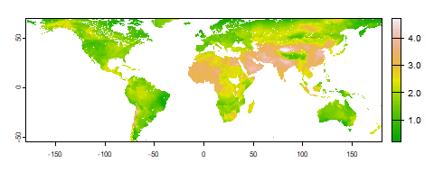
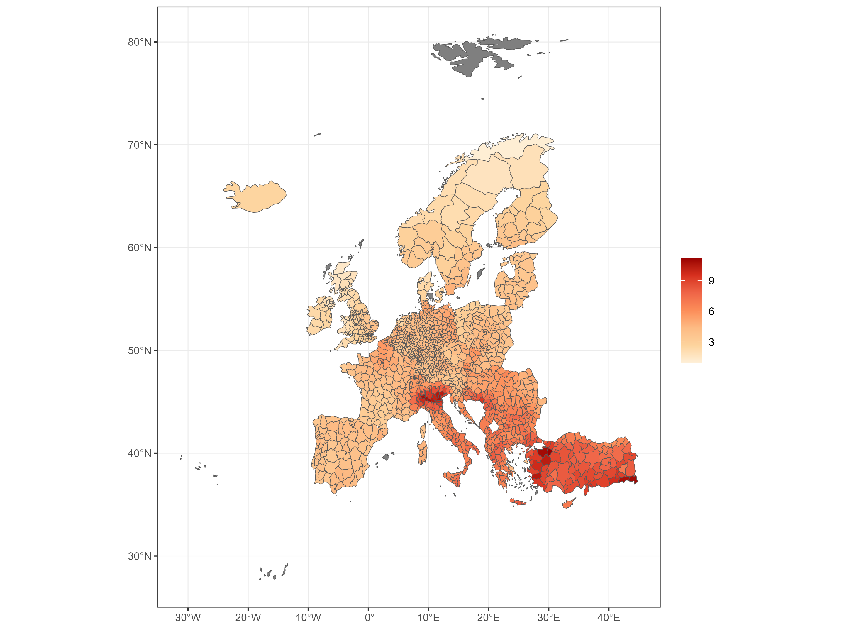
The figures below are an example of the downscaled outputs that can be produced:
Gridded PM2.5 concentration levels for year 2020 (ug/m3, in logarithmic scale)

PM2.5 concentration by NUTS3 region in 2020 (ug/m3)
