Step-by-step example

Step by step example

Introduction

In this example, we analyze the distributional impacts of energy price shocks in Spain, focusing on two scenarios:

• Scenario 1: A price shock affecting fuel prices for private transportation, similar to what occurred during the 2022 energy crisis.
• Scenario 2: A policy intervention where the government implements a measure to reduce domestic energy prices to mitigate the crisis.

We will use the medusa package to evaluate the socioeconomic impacts of these scenarios.

Step 1: Calculate Distributional Impacts by Income Level

Define the Scenarios

1. Download the example file into your working directory by running:

ex_shocks()

2. Locate and open the CSV file “Example_shocks.csv” in your working directory.

3. Each column labeled Scenario__ represents a different scenario. We will keep Scenario 1 and Scenario 2 (but you can also rename them to be more intuitive).

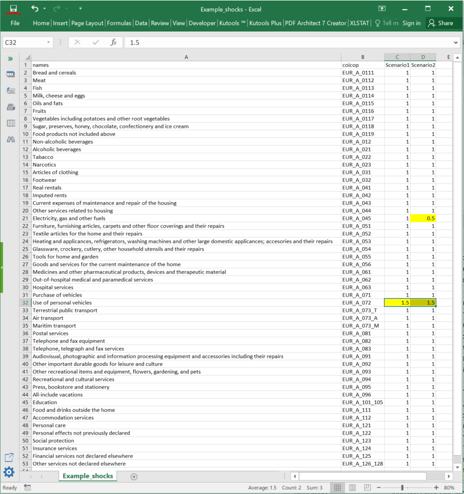
4. Enter the price shocks for each COICOP category and each Scenario. In this case, we introduce:

   • 1.5 in “Use of personal vehicles” for both scenarios to indicate that fuel prices increase by 50%.
   • 0.5 in “Electricity, gas and other fuels” in Scenario 2 to indicate that, due to the government policy, domestic energy prices decrease by 50%.
   • Mantain 1 in all other categories to indicate that prices in these categories remain unaffected.

5. Save the edited CSV file.

6. Upload the edited file into R:

exampledf <- read.csv("Example_shocks.csv", header = TRUE, sep = ",", dec = ".")

Run Distributional Impact Calculation

7. Identify the variables available for distributional impact analysis:

available_var_impact()

This function will return the set of available variables in the console. For this example, we will select “DECILE”, which refers to household income deciles. For more information on available variables, visit here.

8. Compute the distributional impacts by income decile for 2019 data:

calc_di(2019,                      # Base year: 2019
        shocks = exampledf,        # File containing the shocks
        var_impact = "DECILE")     # Select income deciles as the socioeconomic variable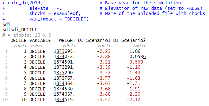

By default, this function saves the produced results and the corresponding figure in your working directory for each specified variable, in this case, for DECILE.

Results Interpretation

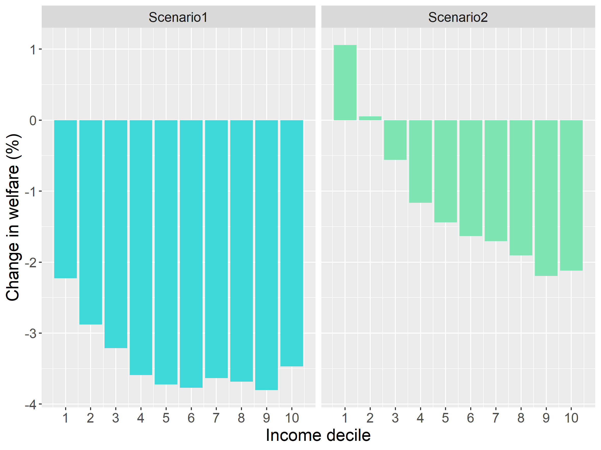
The figure generated by calc_di illustrates the relative impact (%) on total equivalent consumption expenditure (which we use as a proxy of income) across income deciles. A negative change indicates that households are negatively affected, meaning their income decreases by that percentage relative to their previous income. Conversely, a positive change implies a cost reduction, allowing households to save and increase their income by the given percentage.

• In Scenario 1 (left panel), all deciles experience a significant welfare loss, but the impact is higher on middle- and high-income households. This suggests that these households, which rely more on private transportation, are more exposed to fuel price increases.
• In Scenario 2 (right panel), the policy intervention is progressive, as it benefits lower-income households the most while having a smaller impact on higher-income households. This suggests that reducing domestic energy prices mitigates the effects of rising fuel prices, especially for vulnerable groups.

---

Step 2: Calculate Intersectional Distributional Impacts (Income & Gender)

Define Intersectional Variables

9. Download the intersectional variables file into your working directory by running:

ex_var_intersec()

10. Locate and open the CSV file “Var_intersec.csv” in your working directory. Delete the rows for the variables you do not want to analyze. In this case, we will keep the combination QUINTILE-GENDERRP, which represents the household income quintile and the gender of the reference person in the household. For more information on available variables, visit here.

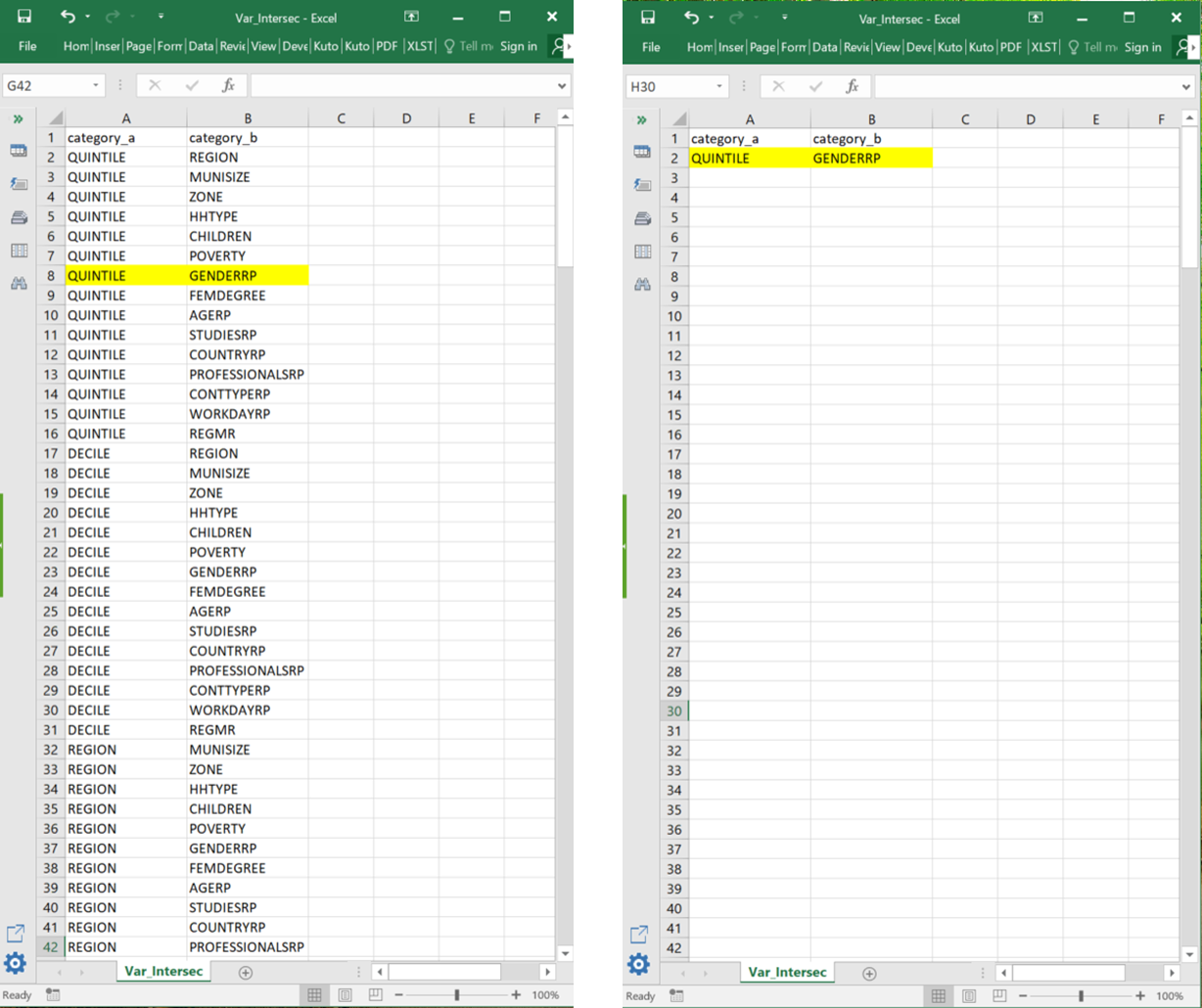
11. Save the edited CSV file and upload it into R:

example_vars <- read.csv("Var_intersec.csv", header = TRUE, sep = ",", dec = ".")

Compute Intersectional Distributional Impacts

12. We will run calc_di similarly to step 8, but in this case, we will disable calculations for individual variables and introduce intersectional variables:

calc_di(2019,                         # Base year: 2019
        shocks = exampledf,           # File containing the shocks
        var_impact = NULL,            # Skip single-variable analysis
        var_intersec = example_vars)  # Use selected intersectional variables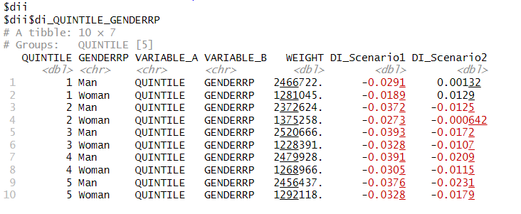

By default, this function saves the produced results and the corresponding figure in your working directory for each specified intersectional variables, in this case, for QUINTILE-GENDERRP.

Results Interpretation

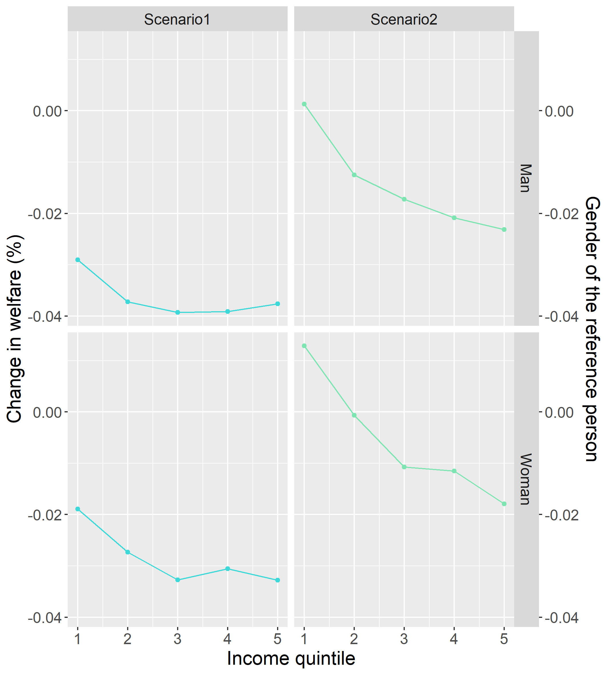
The figure generated by calc_di shows the relative impact (%) on total equivalent consumption expenditure across income quintiles, disaggregated by the gender of the reference person in the household. A negative change indicates a welfare loss, while a positive change implies a cost reduction, improving household welfare.

• In Scenario 1 (left panel), all income quintiles experience a welfare loss, with middle- and high-income households being more affected. The impact is similar across genders, though minor differences exist.
• In Scenario 2 (right panel), the policy intervention is progressive, as it benefits lower-income households the most, while the negative impact remains for higher-income groups. Women-headed households in the lowest quintiles appear to benefit slightly more from the intervention than men-headed households, reinforcing the redistributive nature of the policy.